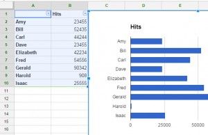
After you’ve entered data into Google Sheets, you may want to create a visualization of that information to make it easier to convey. Luckily, Google Sheets makes it easy for you to convert data into a graph or chart. Easy as Raspberry Pi, if you will.
Google Sheets gives you a variety of options for your graph, so if you want to show parts that make up a whole you can go for a pie chart, and if you want to compare statistics, a bar graph will likely make more sense. Here are our step-by-step instructions for making a graph in Google Sheets.
1. Select cells. If you’re going to make a bar graph like we are here, include a column of names and values and a title to the values.

2. Click Insert.

3. Select Chart.

4. Select which kind of chart. Pie charts are best for when all of the data adds up to 100 percent, whereas histograms work best for data compared over time.

5. Click Chart Types for options including switching what appears in the rows and columns or other kinds of graphs.

6. Click Customization for additional formatting options.

7. Click Insert.

You’ve inserted a graph into your spreadsheet.


